Gridded GDP projections compatible with the five SSPs
October, 2021
Downscaling GDP
Estimated GDPs by 1/12-degree grids during 1850—2100 by 10 year intervals. In the estimation, national GDP data (past data until 2010; future projection under SSPs after 2020) is downscaled considering spatial and economic interactions among cities, urban growth patterns compatible with SSPs, and other auxiliary geographic data (land cover, road network, etc.). Methods which we used are detaily described in our paper and data.
- Daisuke Murakami, Takahiro Yoshida, Yoshiki Yamagata (2021)
Gridded GDP projections compatible with the five SSPs (shared socioeconomic pathways).
Frontiers in Built Environment, 7, 760306.
DOI: 10.3389/fbuil.2021.760306 [LINK] [DATA]
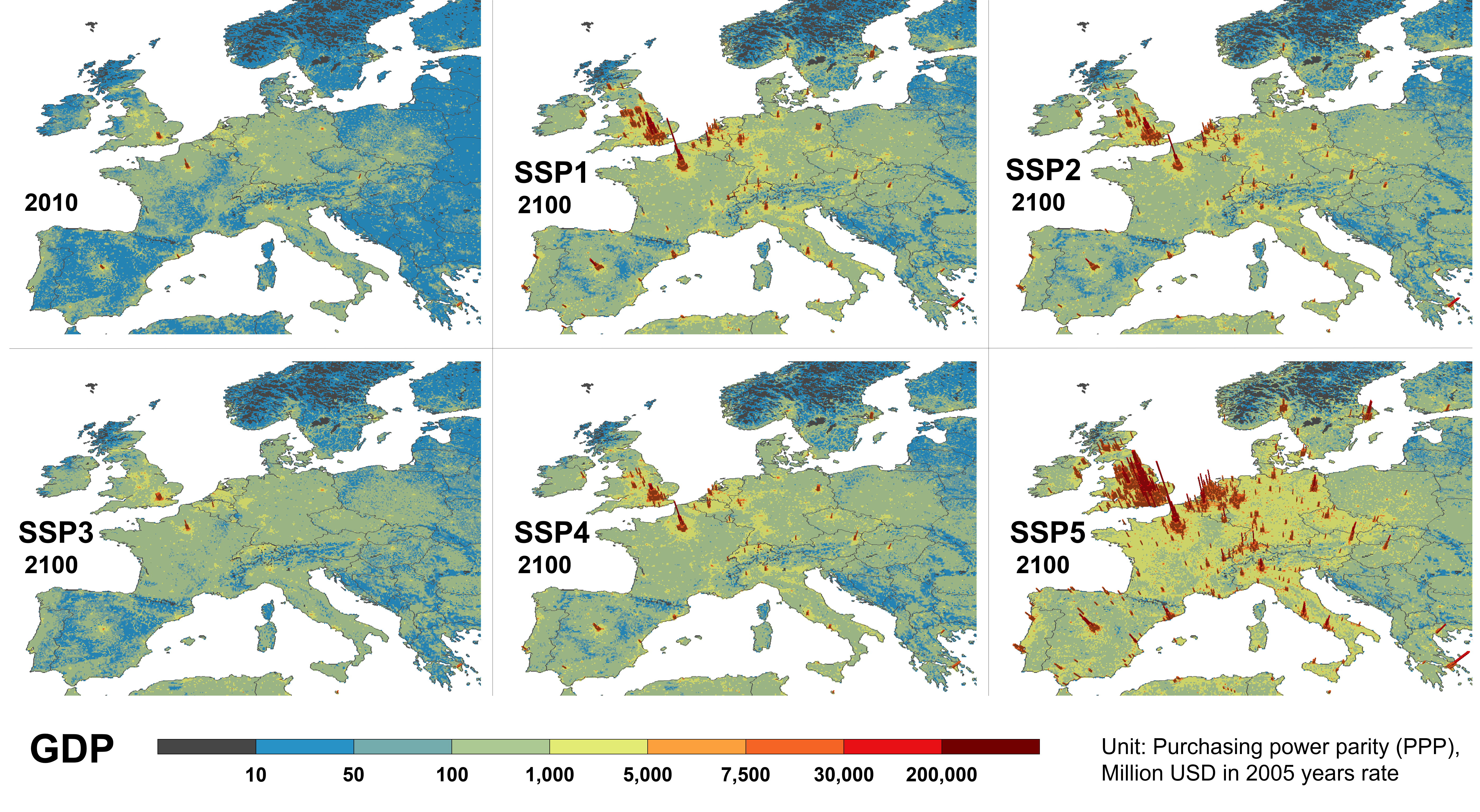
Figure: Europe in 2.5D
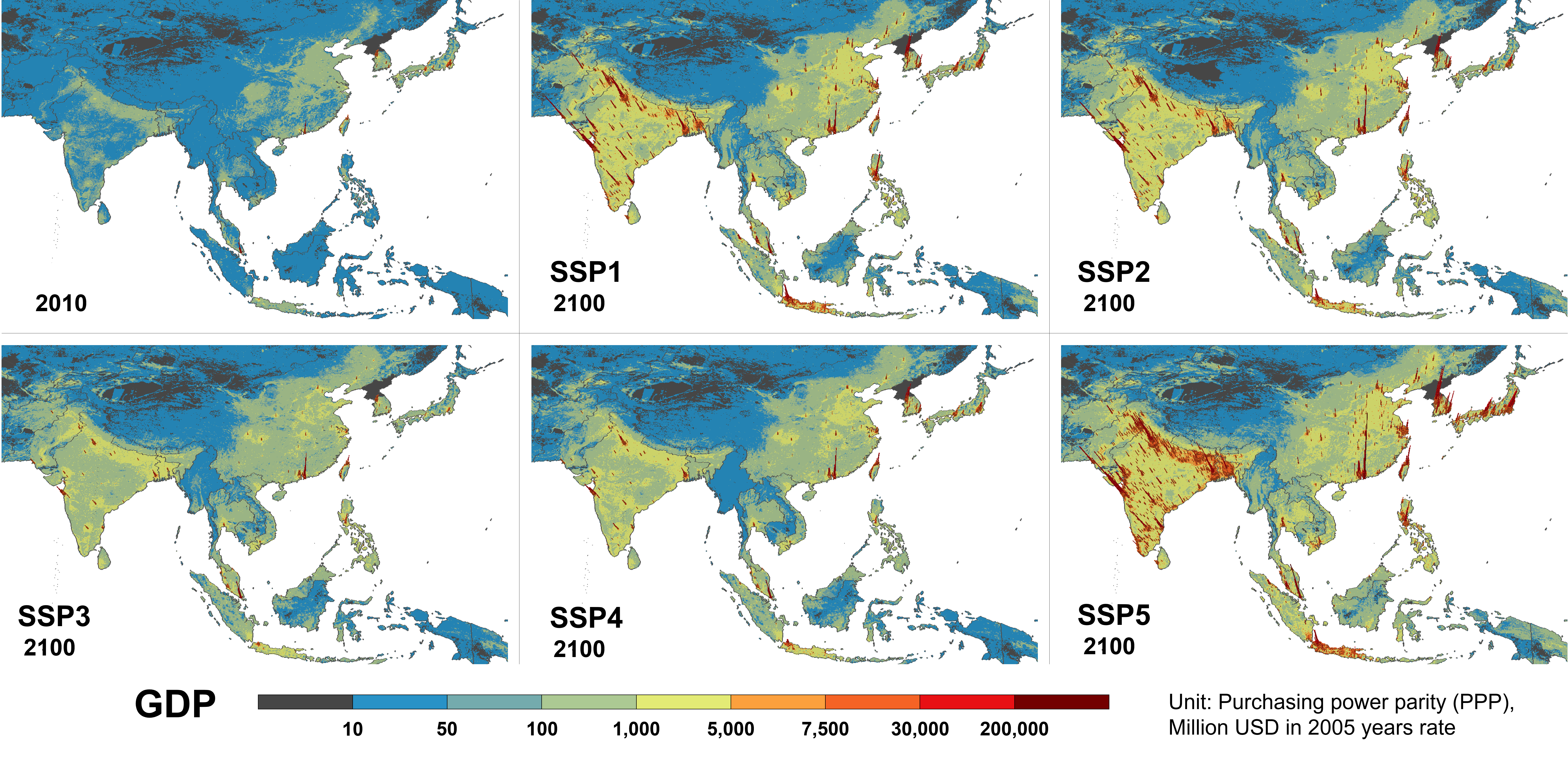
Figure: Asia in 2.5D
Data download
The GDPs for SSP 1–5 between 1850 and 2100 by 10 years are estimated by 2160 x 4320 grids, each of which are 1/12-degree grids, covering the globe. The GDP estimates in each year in each SSP are recorded as a GeoTIff image with resolution of 2160 x 4320. GeoTiff is a Tiff image with spatial coordinates for each grid cell; the coordinates are given by longitude and latitude measured by World Geodetic System 1984 (WGS84).
GeoTiff: [please click here]
Code for visualization
We used R for the 3D globe visualization.
## ------------------
## 3D visualization
## ------------------
library(colorRamps)
library(data.table)
library(dplyr)
library(htmlwidgets)
library(threejs)
library(tidyr)
setwd(****) # please set a directory including the file
dat <- data.table::fread(****) # please wait a moment!
# dat[1:3,]
# longitude latitude gdp
# 1: -36.54172 83.5416 *
# 2: -36.45839 83.5416 *
# 3: -36.37506 83.5416 *
dat <- dat %>%
dplyr::mutate(gdp=if_else(gdp>0,gdp,0)) %>%
dplyr::filter(gdp>0) %>%
dplyr::mutate(gdp.cut=as.numeric(cut(gdp,
breaks=c(0,10^4,10^5,10^6,2.5*10^6,5.0*10^6,
10^7,2.5*10^7,5.0*10^7,10^8,10^9,max(gdp)),
include.lowest=TRUE))) %>%
dplyr::mutate(pid=as.numeric(rownames(.))%%10) %>% # to avoid heavy calculation.
dplyr::filter(pid==0)
3Dglobe <- threejs::globejs(lat=dat$latitude, long=dat$longitude,
val=dat$gdp/10^6, # to adjust bar height
color=colorRamps::matlab.like(11)[dat$gdp.cut],
pointsize=1.6,
atmosphere=F)
3Dglobe